Exercise - Finite Difference Solution - Clay Blanket Sheetpile
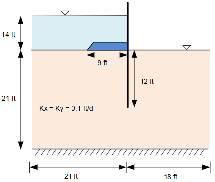
In this exercise, you will implement a finite difference solution to 2D seepage using equations in an Excel file. This problem we will be solving is flow under a sheetpile with a clay blanket on the upstream side of the sheetpile. The problem dimensions and properties are as follows:
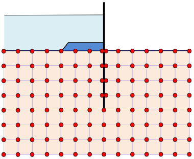
To solve this problem, we will set up a grid with a spacing of 3 ft x 3 ft as follows:
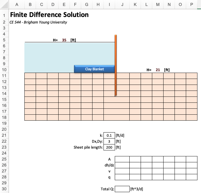
To solve the problem, we will use an Excel file set up as follows:
Download a copy of the file here:
Excel starter file: findiff-1_clayblanket.xlsx
Excel solution file: findiff-1_clayblankey_KEY.xlsx
(a) Fill in the salmon-colored cells with the appropriate formulas to solve the problem using the equations we discussed in class. You should first apply boundary conditions to the upstrem and downstream sides. Then fill in the interior cells using the finite difference equations.
(b) After successfully entering the formulas and iterating, you can use the head values along the exit face to calculate the flow rate out of the system. Enter the formulas to calculate the flow rate using the table at the bottom of the spreadsheet. Assume k = 0.1 ft/day and the head values are in ft. Assume the sheetpile is impermeable and that it is 200 ft long.
Setting up Excel for Dealing with Circular References
When you set up the Excel file, you will have to deal with circular references. The equations are set up so that the head values are calculated based on the head values in the adjacent cells. This will create a circular reference. To deal with this, you will need to do the following before entering your formulas:
- Go to the File menu and select Options.
- In the Excel Options dialog box, select Formulas.
- Check the box for Enable iterative calculation.
- Set the maximum iterations to 100 and the maximum change to 0.0001.
- Turn on the box for Manual calculation.
- Click OK.
Now you can enter your formulas and use the Calculate Now button on the Formulas ribbon to recalculate the sheet. You can also hit the F9 button to recalculate the sheet.
To track down minor errors
If you are getting values from your formulas but they don't look right, you can often track down the cells with errors using conditional formatting. (a) Go to the Home tab and click on Conditional Formatting. (b) Select the Color Scales option and pick a color scale. (c) The color gradation should be smooth. If you see a discontinuity, check the associated formula.
To fix major errors
If you have an error in your equations or if you attempt the calculations before all of the equations are properly entered, you may encounter a situation where the formulas return an error message such as #NUM. At this point you will be stuck because all of the adjacent formulas will be in error as well. To solve this problem you can try the following:
(a) Select the entire problem domain corresponding to the colored text where you are solving the finite difference equations and copy the equations to the clipboard.
(b) Paste the entire set of equations at some other location on the spreadsheet such as starting at row 34.
(c) For each of the cells that are displaying an error message, type in a new value such as the average of the upstream head of the downstream head. Note that this will overwrite the existing equation. Make sure that when you type a new value in for the cells that are merged underneath the tip of the sheet pile that you don't unmerge the cells.
(d) Select the entire range that you pasted as part of step (a) and paste them back into the original cells using the Paste Special/Paste Formulas command. When you paste the cells it should automatically trigger recalculation but it will use the new values you entered in step (c). If your formulas are correct this should fix the problem.