Exercise - Well Equations

Part 1 - Radius of Influence

The radius of influence of a well is the distance from the well at which the drawdown is negligible. The radius of influence can be estimated using the following equations:

Name	Type	Equation
Lembke	Semi-Empirical	\(R = H\sqrt{\frac{k}{2N}}\)
Weber	Semi-Empirical	\(R = 2.45\sqrt{\frac{Hkt}{n_e}}\)
Kusakin	Semi-Empirical	\(R = 1.9\sqrt{\frac{Hkt}{n_e}}\)
Siechardt	Empirical	\(R = 3000s_w\sqrt{k}\)
Kusakin	Empirical	\(R = 575s_w\sqrt{\frac{H}{k}}\)

Where:

H = initial thickness (B for confined aquifers, h for unconfined aquifers) [m]
k = hydraulic conductivity [m/sec]
\(s_w\) = drawdown at the well [m]
\(n_e\) = effective porosity (storativity S, for confined) [-]
t = time since pumping began [sec]
N = accretion from rainfall [m/sec]

The following spreadsheet a sample set of calculations for each of the equations above.

Excel file: radius_of_influence.xlsx

Part 2 - Confined Aquifer

In this exercise, you will calculate the water level at the center of the well and as a function of distance from the well for a confined aquifer.

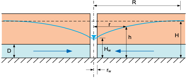
The following equations can be used to calculate the head (h) as a function of distance (x) from the well:

\(h = H = \dfrac{q}{2\pi k D} \ln\left(\dfrac{r}{R}\right)\)

Where:

h = head [L]
H = initial head prior to pumping [L]
q = flow rate [L³/T]
k = hydraulic conductivity [L/T]
D = thickness of the confined aquifer [L]
r = distance from the well [L]
R = radius of influence of the well [L]

Assume the following values for the confined aquifer:

Parameter	Value	Units
H	50	m
Q	0.2	m³/s
k	1e-3	m/s
D	15	m
R	500	m
\(r_w\)	0.1	m

a) Calculate the head at the center of the well (r = \(r_w\)).

b) Let r vary from rw to R. Calculate and plot the head as a function of distance (r) from the well.

Excel starter file: confined.xlsx

Excel solution file: confined_KEY.xlsx

Python starter file:

Python solution file:

Part 3 - Unconfined Aquifer

In this exercise, you will calculate the water level at the center of the well and as a function of distance from the well for an unconfined aquifer.

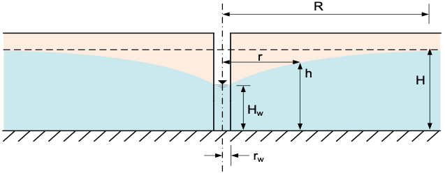
The following equations can be used to calculate the head (h) as a function of distance (x) from the well:

\(h = \sqrt{H^2 - \dfrac{q \ln\left(\dfrac{R}{r}\right)}{\pi k} }\)

Where:

h = head [L]
H = initial head prior to pumping [L]
q = flow rate [L³/T]
R = radius of influence of the well [L]
r = distance from the well [L]
k = hydraulic conductivity [L/T]

Assume the following values for the unconfined aquifer:

Parameter	Value	Units
Q	0.2	m³/s
k	1	cm/s
H	50	m
R	500	m
\(r_w\)	0.1	m

a) Calculate the head at the center of the well (r = \(r_w\)).

b) Let r vary from rw to R. Calculate and plot the head as a function of distance (r) from the well.

Excel starter file: unconfined.xlsx

Excel solution file: unconfined_KEY.xlsx

Python starter file:

Python solution file: